YMatrix
Quick Start
Connecting
Benchmarks
Deployment
Data Usage
Data Ingestion
Data Migration
Data Query
Manage Clusters
Upgrade
Global Maintenance
Expansion
Monitoring
Security
Best Practice
Technical Principles
Data Type
Storage Engine
Execution Engine
Streaming Engine(Domino)
MARS3 Index
Extension
Advanced Features
Advanced Query
Federal Query
Grafana
Backup and Restore
Disaster Recovery
Graph Database
Introduction
Clauses
Functions
Advanced
Guide
Performance Tuning
Troubleshooting
Tools
Configuration Parameters
SQL Reference
The previous section introduced how MatrixDB models time-series data. As a distributed database, MatrixDB differs from standalone databases in terms of data storage. This section explains the distributed architecture of MatrixDB and how to design table distribution strategies based on this architecture.
For the accompanying video tutorial, refer to MatrixDB Data Modeling and Spatio-Temporal Distribution Model
MatrixDB is a distributed database with a centralized architecture, consisting of two types of nodes: master and segment.
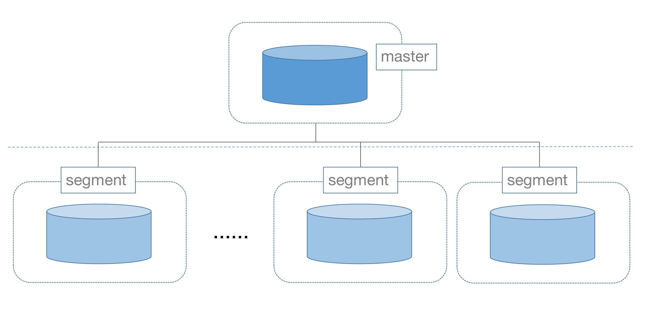
The master is the central control node responsible for receiving user requests and generating query plans. It does not store data. Data is stored on segment nodes.
There is only one master node, while the number of segment nodes is at least one and can scale up to dozens or even hundreds. More segment nodes enable higher storage capacity and stronger computational power.
MatrixDB supports two data distribution methods across segments: sharding and replication. Sharding further divides into hash and random distribution:
In sharded distribution, data is horizontally partitioned, with each row stored on only one segment. In hash sharding, one or more distribution keys are specified. The database computes a hash value over these keys to determine the target segment. Random sharding assigns rows to segments randomly.
In replicated distribution, the entire table is duplicated across all segment nodes. Every segment stores all rows. This method consumes significant storage space and is typically used only for small tables that frequently participate in join operations.
In summary, there are three distribution strategies. You can specify the strategy when creating a table using the DISTRIBUTED BY clause:
DISTRIBUTED BY (column)DISTRIBUTED RANDOMLYDISTRIBUTED REPLICATED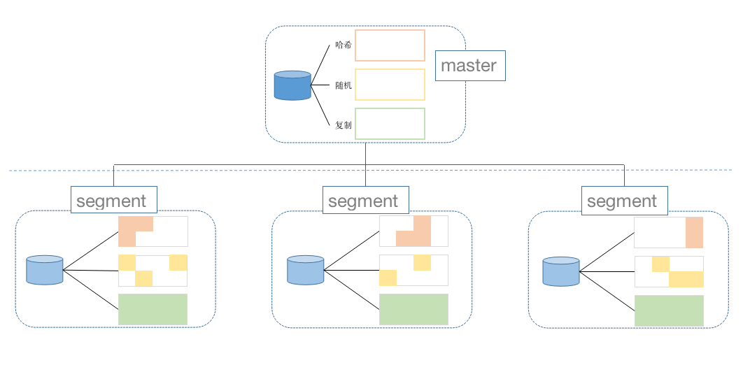
In MatrixDB’s distributed architecture, most tables use sharded storage, yet full relational queries are supported. From the user's perspective, it behaves like a PostgreSQL instance with virtually unlimited capacity.
How are joins across segments handled? MatrixDB uses a Motion operation. When data involved in a join resides on different segments, Motion moves the required data to the same segment for processing.
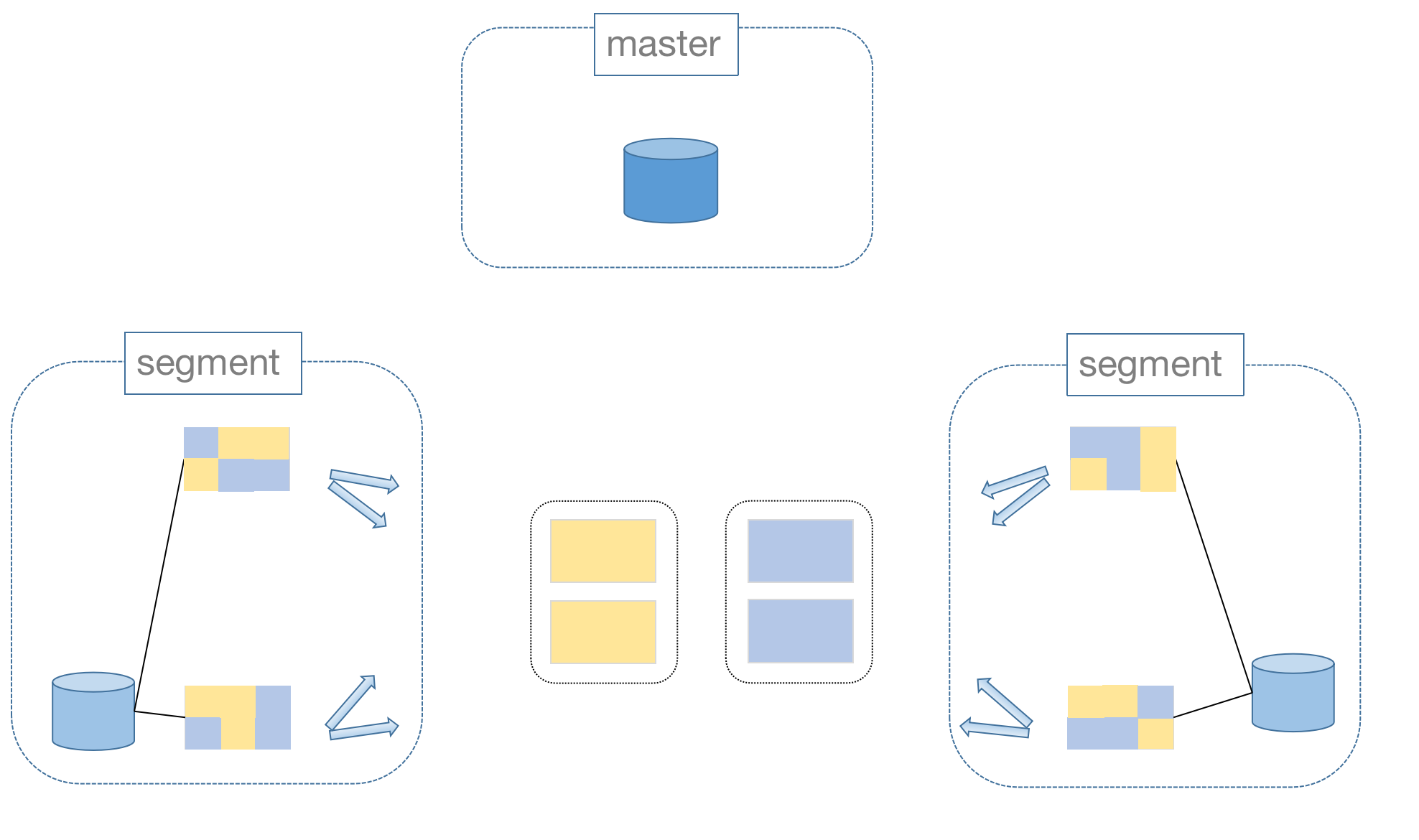
However, Motion incurs overhead. Therefore, when designing tables, carefully consider both the data distribution pattern and the expected query workload.
Motion can be avoided only when all data involved in a join already resides on the same segment. Hence, for large tables frequently joined, it is best practice to set the join key as the distribution key.
Now that we understand MatrixDB’s distribution methods and their trade-offs, let’s discuss optimal distribution strategies for time-series tables.
Consider the metrics table first. Metric data volumes are typically very large, making replicated distribution impractical. Random distribution lacks predictability and hinders efficient analysis. Therefore, hash distribution is preferred.
Which column should be chosen as the distribution key?
Time-series data has three main dimensions:
Most analytical queries group by device and join with attributes from the device table. To align data placement with query patterns, use Device ID as the distribution key.
The device table has a relatively fixed size and does not grow indefinitely like metric data. Therefore, replicated distribution is recommended. This ensures that joins with the metrics table do not require inter-segment data movement, improving performance.