Introduction

In large-scale analytical databases, parallel scanning usually means that more computing resources participate in processing. Therefore, in theory, queries should run faster.

However, in real-world scenarios, query performance depends not only on whether scanning itself is fast, but also on whether data needs to be “moved.” In many cases, scanning is already fast enough. What actually slows down queries is the movement of intermediate data during execution, additional redistribution, and the resulting increase in execution path complexity.

The goal of MARS3 Bucket is to address this problem. It is not simply about splitting data into smaller chunks, nor is it a traditional logical bucketing mechanism. Instead, it is a data organization approach that enables better coordination between parallel scanning and local computation, so that after parallel scanning, data can still maintain good locality. This reduces unnecessary data movement and makes it easier for the benefits of parallelism to be reflected in end-to-end query performance.

Tests show that after adopting MARS3 Bucket, performance in complex analytical query scenarios, such as TPCH and TPCDS, has doubled compared to the previous version of YMatrix.

Related Concepts

Before understanding the root cause of the problem, we need to clarify two concepts: data co-locality and parallel scanning.

Data Co-locality

In the YMatrix database, data is distributed across multiple data nodes (segments) according to specific rules, and the data on all data nodes together constitute a complete dataset.

Each table must define a distribution key. During data insertion, a hash value is computed based on this key, and the result determines which data node the data is stored on. Therefore, when tables share the same distribution key, identical key values are guaranteed to reside on the same data node.

As a result, operations such as JOIN and GROUP BY based on the distribution key can be executed locally with maximum efficiency, without requiring data movement. This phenomenon is referred to as data co-locality.

Parallel Scanning

First, YMatrix adopts an MPP (Massively Parallel Processing) architecture. From the perspective of the entire table, all data nodes scan simultaneously, which naturally constitutes parallel execution at the cluster level.

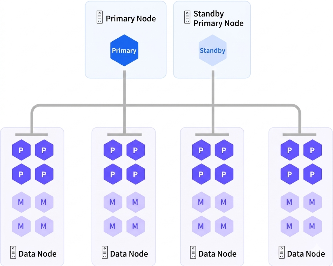
Another level of parallelism exists within a single node. From the perspective of a specific data node, multiple processes can participate in scanning the data within that node. This is referred to as intra-node parallelism.

Why Parallel Scanning Does Not Necessarily Make Queries Faster

Returning to the question itself, why does parallel scanning not necessarily make queries faster?

First, parallel scanning itself introduces certain costs, such as coordination among multiple scanning processes, data exchange between them, as well as the overhead of process creation and management.

In distributed databases, the situation becomes more complex. Query performance depends not only on the scanning itself, but also on whether the data can continue to be computed “in place” after the scan.

As mentioned earlier, if a table has already been hash-distributed by a certain distribution key, then operations such as GROUP BY and JOIN based on this key can be completed locally. This is because rows with the same key value naturally reside on the same data node. The master node only needs to wait for each data node to complete its computation and then perform the final aggregation.

However, once parallel scanning is introduced, the situation becomes somewhat more complex. Parallel scanning focuses on having multiple scanning processes read data together, but it does not inherently guarantee that rows with the same key value remain grouped together. This is because parallel scanning typically assigns tasks based on page blocks or scan ranges.

As a result, once rows with the same key value are processed by different scanning processes, additional data transfer is required in subsequent steps to complete correct aggregation or joins. Thus, work that could originally be completed locally becomes “parallel scan → data reshuffling → continue computation.”

Let us look at a concrete example. Suppose a data node contains four rows with values 1, 2, 2, and 3, and each row resides on a separate data page.

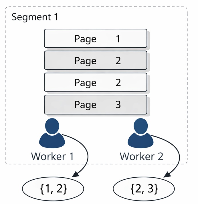
Assume that two workers participate in the scan: worker1 scans the rows with values 1 and 2, while worker2 scans the rows with values 2 and 3. In this case, it cannot be guaranteed that the same value (in this example, 2) is exclusively produced by a single worker.

Therefore, to ensure consistency and correctness of the results, these scattered intermediate results must be re-collected and redistributed before further computation. As a result, the database needs to transfer the results for value 2 again to a data node for processing.

It is easy to imagine that if the amount of data to be transferred reaches tens of thousands, millions, or even tens of millions of rows, the cost of such “data movement” will be extremely significant, and the entire execution path will become longer and more complex.

Therefore, from the user’s perspective, this leads to a very practical issue: parallelism is enabled and CPU utilization increases, but intermediate data movement also increases, and overall query performance may not necessarily improve.

What Is MARS3 Bucket

To address the above problem, MARS3 Bucket was introduced. MARS3 Bucket is not a simple bucketing feature, nor is it a logical partitioning mechanism at the syntax level. Its core objective is to ensure that after parallel scanning, data can still maintain strong locality, so that more computation can continue to be completed locally.

If traditional distribution determines which data node the data is placed on, then MARS3 Bucket goes one step further on top of that: it not only determines which data node the data is placed on, but also further organizes the data into more structured buckets within that node.

As a result, when multiple processes scan data concurrently, the mechanism is no longer simply “whichever process grabs a page scans that page,” but instead “each worker scans a specific set of buckets it is responsible for.” This is the most fundamental difference compared to conventional parallel scanning.

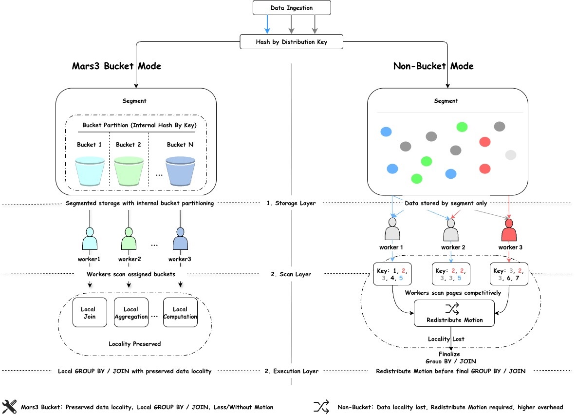
Under the MARS3 Bucket model, data within a data node is first organized into more structured buckets. During scanning, multiple workers process different buckets respectively. Since the mapping from keys to buckets is deterministic, data with the same key is more likely to flow along the same processing path.

In this way, downstream operators can more easily complete computation locally, without requiring another round of data movement. For users, the most intuitive benefit is that parallelism is no longer only applied to “scanning,” but is effectively extended to “computation.”

Example

Let us look at an example. Suppose there is a table t_sales with distribution key c1. Consider the following SQL: SELECT c1, COUNT(*) FROM t_sales GROUP BY c1;The SQL is straightforward: group by c1 and count the number of rows for each value of c1.

In the case of non-parallel scanning, after each data node completes a local sequential scan, it directly performs hash aggregation. Since the table itself is distributed by c1, at the data node level it can be guaranteed that rows with the same c1 value reside on the same node, and no cross-node data transfer is required. After each node completes local aggregation, the result is already globally correct, and only a final aggregation on the master node is needed.

Execution plan:

Gather Motion 4:1
  -> HashAggregate
       Group Key: c1
       -> Seq Scan on t_sales

However, once parallel scanning is enabled, the execution plan becomes as follows:

Gather Motion 12:1
  -> Finalize HashAggregate
       Group Key: c1
       -> Redistribute Motion 12:12
            Hash Key: c1
            -> Partial HashAggregate
                 Group Key: c1
                 -> Parallel Seq Scan on t_sales

Since workers read data by competing for pages (i.e., randomly acquiring pages to scan), from the optimizer’s perspective, it can no longer guarantee that each c1 value is exclusively produced by a single worker.

Therefore, in the second step (Partial HashAggregate), each worker first performs local aggregation on the data it scans. In the third step (Redistribute Motion with hash key c1), data movement is introduced. This is because after partial aggregation, the same c1 value may still exist in the intermediate results of multiple workers, and must be redistributed by c1 to ensure final correctness.

In short, the issue is not the table’s distribution strategy, but that the parallel scan path does not preserve the distribution semantics required for upper-level aggregation. To compensate for this, the optimizer has to insert an additional Redistribute Motion operator, which is exactly the root cause of parallelism benefits being eroded.

With MARS3 Bucket, the execution plan becomes:

Gather Motion 12:1
  -> HashAggregate
       Group Key: c1
       -> Parallel Custom Scan (MxVScan)

Because data is organized by buckets, each worker scans one or more buckets during execution. In this way, the scan output can continue to preserve distribution characteristics and retain distribution semantics. As a result, there is no need to explicitly introduce a Redistribute Motion operator in the execution plan, and no data movement is required.

Each data node completes computation locally, and the results are then aggregated upward. Combined with parallelism, CPU resources can be fully utilized, significantly improving SQL execution efficiency.

How to Use MARS3 Bucket

Syntax:

CREATE TABLE foo (c1 INT, c2 INT)
USING mars3
WITH (mars3options='nbuckets = 2');

• nbuckets ranges from 1 to 128
• Default value is 1 (no bucketing)

Best Practices

The goal of buckets is to provide each worker within a segment with its own data to scan.

Recommended configurations:

Table size < 50 GB

No bucketing (nbuckets = 1) Suitable for dimension tables and small datasets with infrequent large queries

50 GB – 500 GB

Start with nbuckets = 4 or 8 Suitable for large fact tables with frequent aggregations and complex queries

500 GB – 2 TB

Use nbuckets = 8 or 16 Matches common intra-node parallelism without excessive complexity

2 TB

Choose between 16 or 32 based on actual parallelism and benchmarking results

Core Value of MARS3 Bucket

Reduce Unnecessary Data Movement

In distributed query scenarios, many slow queries are not due to the computation itself, but rather to the data movement. MARS3 Bucket minimizes unnecessary redistribution, allowing more processing to be completed locally.

Simplify Execution Pipelines

With less data movement, execution paths become simpler. For complex analytical SQL, benefits extend across the entire pipeline: fewer intermediate steps, less scheduling overhead, and lower processing cost.

Make Parallelism Truly Improve End-to-End Performance

Faster scanning does not automatically mean faster queries. MARS3 Bucket ensures that parallelism extends beyond scanning and translates into real performance gains across the entire query execution path.

Conclusion

In MPP query scenarios, the most expensive factor is often not scanning or computation itself, but data transfer during execution.

If parallel scanning fails to preserve data distribution semantics, increased compute power can easily translate into more data movement rather than higher query efficiency.

The significance of MARS3 Bucket lies in avoiding this situation. It transforms parallel scanning from simply “more processes reading data” into a more structured and efficient intra-node parallel processing model, effectively extending parallelism into computation.

For large-scale analytical workloads that rely on local aggregation and joins, this means less data movement, fewer execution fragments, and a higher possibility of converting parallelism into real end-to-end performance gains—ultimately reducing overall usage costs for users.