In real-world scenarios, customer data systems are rarely purely OLTP or purely OLAP. Under hybrid workloads, traditional storage systems often naturally diverge: some engines excel at scanning and compression but struggle with sustained small writes and updates; others are fast for writes and stable for point queries but incur high costs and low efficiency for full table scans and aggregations. When we attempt to assemble multiple systems into so-called HTAP, we introduce challenges related to data freshness, resource isolation, operational complexity, and overall cost. Therefore, we developed MARS3: a storage engine designed for AP-core hybrid workloads. Its goal is not to be a universal replacement for everything, but to handle the most common and critical hybrid workloads customers face within a single, manageable storage system, ensuring performance and stability under high pressure through explainable mechanisms.
If you are evaluating options and solutions, it is recommended to read Chapters 1-2 first to understand the applicability boundaries. If you are an architect or DBA, focus on Chapters 3-6 to understand the mechanisms and trade-offs. If you are responsible for delivery and operations, Chapter 7 provides a fast path from symptoms to resolution, including templates.
MARS3 targets AP-core hybrid workloads – prioritizing scan and aggregation efficiency, stability under continuous writes, and the experience of detailed data lookups in common scenarios. However, MARS3 does not aim to be excellent in all dimensions, such as extreme pure TP or ultra-high-frequency, large-range updates.
In most customer systems, data is not written first and then analyzed later; writing and usage happen concurrently, with increasingly stringent business requirements for real-time capabilities. Businesses want data to be as fresh as possible: production line device data, once written, should immediately form a production dashboard; vehicle status updates in telematics should instantly trigger alerts and analysis; sensor data entering an IoT platform should support real-time trend analysis and anomaly detection. Simultaneously, operations and R&D teams need to perform detailed data lookups at any time, such as locating original records for a specific device, vehicle, or workstation within a certain time period, and then perform aggregations, correlation analysis, or multi-table joins based on that.
The common characteristic of these scenarios is that the workload is mixed and predominantly analysis-oriented with continuous writes. The write side could involve batch imports (historical backfill, daily batch settlements), continuous micro-batches (T+0, minute-level aggregations), or even sporadic point writes and corrections. The query side includes global summary reports, filtered scans, and high-frequency lookups on single entities.
Therefore, the essence of this contradiction is not choosing between fast writes or fast queries, but whether the system can maintain both analysis efficiency and efficient, stable write performance when continuous writing and continuous analysis coexist.
In hybrid workloads, the problem is often not that a specific system is inherently good or bad, but that different storage formats excel in inherently different directions.
Row-store is the most classic storage method for traditional databases like PostgreSQL, MySQL, etc. It stores each complete row of data together, like individual "whole packages." Systems that excel with row-store/transactional paths are suitable for detailed lookups and retrieving small numbers of records by primary key/conditions. However, once analytical queries arise (using only a few columns, scanning large amounts of data for filtering/aggregation), the system often has to read the entire row, even if most columns are unused. The results are:
Reading many unnecessary columns consumes disk and cache bandwidth.
Scans and aggregations become slower, consuming more resources for the same analysis.
As data volume grows, this invalid I/O becomes more pronounced and costly.
Columnar storage, to achieve high scan efficiency and high compression ratios, typically requires stronger data organization and metadata maintenance. Data is stored in blocks by column, relying on encoding, dictionaries, statistics, etc., to enhance processing efficiency (e.g., Clickhouse, HBase). Under this architecture, writes often involve more than just appending records; they entail additional structured maintenance:
Write Amplification: A single logical write can introduce multiple physical writes (multiple column blocks, metadata, etc.), with background processes like merging/rewriting needed to maintain data organization quality.
Amplification Effect of Small Batches: When writes become high-frequency micro-batches or continuous small batches, the fixed overhead per write unit is higher, merging/rewriting becomes more frequent, leading to greater maintenance pressure in the long run.
Coupling with Updates and Deletes: Columnar storage often handles UPDATE/DELETE via versioning/marking/rewriting to consolidate garbage. If the proportion of updates/deletes rises and background management is insufficient, space amplification can occur, and the read path can lengthen (needing to process more invalid versions/fragmented blocks).
Thus, columnar storage is well-suited for read-heavy, large-scale analytical scans, but under hybrid workloads, its requirements for the write path and background management are significantly higher.
Placing writes in one system and analytics in another, then connecting them via synchronization/ETL, can theoretically achieve the advantages of both sides. However, the common costs in reality are: data must be "moved," and the longer the pipeline, the harder it is to achieve sufficient freshness; the more systems involved, the more complex it becomes to maintain consistent definitions, perform data backfilling and reconciliation, handle failure recovery, and manage permissions and monitoring, ultimately leading to higher overall costs.
On the surface, customer requirements like "fast writes, fast queries, and low cost" seem contradictory. However, from an engineering perspective, hybrid workloads are not evenly distributed. In most businesses, the core value of the system still lies in producing analytical results (reports, metrics, diagnostics, insights). Writes and detailed lookups serve more to ensure data continuously enters and is readily available. Therefore, MARS3's design trade-offs are clear: it targets hybrid workloads but establishes a manageable storage system centered on AP as the primary battlefield, focusing on analysis efficiency and stability under continuous writes:
As data scale grows and concurrency increases, the system should be able to complete analytical queries with less invalid I/O, better data skipping, and higher throughput. It pursues "maximizing output per unit resource," making broad table scans and periodic statistics more controllable.
Supports various write patterns, from batch imports to continuous micro-batches (T+0), ensuring the system remains predictable under the normal state of "continuous writes, continuous queries." Background maintenance (like merging/reclamation) must be manageable, not randomly impacting online queries.
Provides adequate access paths and experience for common real-world needs like single-entity lookups, time-range queries, and conditional filtering, avoiding a system disconnect where "analytics are strong, but lookups feel disjointed."
MARS3 adopts an LSM-Tree style data organization: the write side quickly absorbs data and performs sequential writes to disk; the read side emphasizes data skipping and scan efficiency enabled by ordered data; background maintenance processes gradually evolve data from write-friendly to read-friendly forms.
Within this system, there are three core objects: Run and Level (which determine how data is segmented and layered), RowStore and ColumnStore (how the physical layout of data balances writes and reads), and Delta and MVCC (how updates/deletes are represented, why amplification occurs, and how it is reclaimed). These will be introduced sequentially.
Data stored in MARS3 is ordered. A contiguous segment of ordered data is called a Run.
In products like RocksDB/LevelDB, the files containing ordered data are called SSTs. In YMatrix, a RUN is another term for SST.
Runs are of two types. To enable high-speed writes, inserted data is first stored as a RowStore Run. Subsequently, to facilitate reading and compression, we convert RowStore Runs into ColumnStore Runs. A single Run has a size upper limit:
Table-level parameter max_runsize, used to specify the maximum size of a single RUN when creating a table. Max 16384 MB.
Default is 4096 MB.
We can use the matrixts_internal.mars3_files function to view the extension files and delta files of MARS3 tables. These mainly include DATA, LINK, FSM, DELTA. If the table has indexes, corresponding INDEX files will also exist:
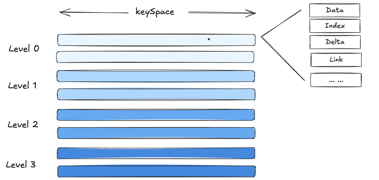
DATA: Main data files, storing user data.
FSM: Stands for Free Space Map. In YMatrix, update and delete operations do not operate on the original data space in-place. Instead, they use a multi-version approach for tuples. This leads to "expired data" – when a version of a tuple is no longer visible to any transaction, it is expired, and the space it occupies can be freed. FSM files track these available spaces for efficient allocation when needed.
LINK: Used during update and delete operations to maintain the relationship between upstream and downstream tuple versions during compaction.
DELTA: Stores deletion information. MARS3 does not modify data in place for updates and deletions. Instead, it relies on DELTA files (containing deletion info like XMAX) and version information to mask old data, thereby controlling data visibility.
INDEX and INDEX_1_TOAST: Store index files. MARS3 currently supports BRIN and BTREE indexes.
postgres=# select * from matrixts_internal.mars3_files('test');
 segid | level | run |     file      | seq |            path            |  bytes
-------+-------+-----+---------------+-----+----------------------------+---------
     1 |     0 |   1 | DATA          |   0 | base/14011/235713_meta_1.2 | 1081344
     1 |     0 |   1 | DELTA         |   0 | base/14011/235713_meta_1   |   32768
     1 |     0 |   1 | LINK          |   0 | base/14011/235713_meta_1.1 |       0
     1 |     0 |   1 | FSM           |   0 | base/14011/235713_meta_1.3 |  131072
     1 |     0 |   1 | INDEX_1       |   0 | base/14011/235713_meta_1.4 |   65536
     1 |     0 |   1 | INDEX_1_TOAST |   0 | base/14011/235713_meta_1.5 |       0
     2 |     0 |   1 | DATA          |   0 | base/14011/253866_meta_1.2 | 1081344
     2 |     0 |   1 | DELTA         |   0 | base/14011/253866_meta_1   |   32768
     2 |     0 |   1 | LINK          |   0 | base/14011/253866_meta_1.1 |       0
     2 |     0 |   1 | FSM           |   0 | base/14011/253866_meta_1.3 |  131072
     2 |     0 |   1 | INDEX_1       |   0 | base/14011/253866_meta_1.4 |   65536
     2 |     0 |   1 | INDEX_1_TOAST |   0 | base/14011/253866_meta_1.5 |       0
     3 |     0 |   1 | DATA          |   0 | base/14011/243459_meta_1.2 | 1081344
     3 |     0 |   1 | DELTA         |   0 | base/14011/243459_meta_1   |   32768
     3 |     0 |   1 | LINK          |   0 | base/14011/243459_meta_1.1 |       0
     3 |     0 |   1 | FSM           |   0 | base/14011/243459_meta_1.3 |  131072
     3 |     0 |   1 | INDEX_1       |   0 | base/14011/243459_meta_1.4 |   65536
     3 |     0 |   1 | INDEX_1_TOAST |   0 | base/14011/243459_meta_1.5 |       0
     0 |     0 |   1 | DATA          |   0 | base/14011/238674_meta_1.2 | 1081344
     0 |     0 |   1 | DELTA         |   0 | base/14011/238674_meta_1   |   32768
     0 |     0 |   1 | LINK          |   0 | base/14011/238674_meta_1.1 |       0
     0 |     0 |   1 | FSM           |   0 | base/14011/238674_meta_1.3 |  131072
     0 |     0 |   1 | INDEX_1       |   0 | base/14011/238674_meta_1.4 |   65536
     0 |     0 |   1 | INDEX_1_TOAST |   0 | base/14011/238674_meta_1.5 |       0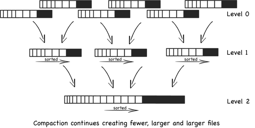
(24 rows) MARS3 organizes data based on the LSM-TREE concept. Individual Run files are organized into Levels, with a maximum of 10 levels: L0, L1, L2... L9. When the number of Runs in a level reaches a certain threshold, or the total size of multiple Runs in the same level exceeds a threshold, a merge is triggered. These Runs are merged into a single Run and promoted to a higher level. To accelerate Run promotion, multiple merge tasks are allowed to execute concurrently within the same level.
In YMatrix, a certain number of background merge processes periodically check the state of each table and perform merge operations.
YMatrix provides the matrixts_internal.mars3_level_stats utility function to view the status of each level in a MARS3 table. This is useful for evaluating table health, such as checking if Runs are merging as expected, if there are too many invisible Runs, and if Run counts are within normal ranges.
postgres=# select * from matrixts_internal.mars3_level_stats('test') limit 10;
 segid | level | total_nruns | visible_nruns | invisible_nruns | object_nruns | object_visible_nruns | level_size
-------+-------+-------------+---------------+-----------------+--------------+----------------------+------------
     1 |     0 |           1 |             1 |               0 |            0 |                    0 | 1280 kB
     1 |     1 |           0 |             0 |               0 |            0 |                    0 | 0 bytes
     1 |     2 |           0 |             0 |               0 |            0 |                    0 | 0 bytes
     1 |     3 |           0 |             0 |               0 |            0 |                    0 | 0 bytes
     1 |     4 |           0 |             0 |               0 |            0 |                    0 | 0 bytes
     1 |     5 |           0 |             0 |               0 |            0 |                    0 | 0 bytes
     1 |     6 |           0 |             0 |               0 |            0 |                    0 | 0 bytes
     1 |     7 |           0 |             0 |               0 |            0 |                    0 | 0 bytes
     1 |     8 |           0 |             0 |               0 |            0 |                    0 | 0 bytes
     1 |     9 |           0 |             0 |               0 |            0 |                    0 | 0 bytes
(10 rows)
Based on experience:
When level = 0, if the number of runs > 3, the state is unhealthy.
When level = 1, if the number of runs > 50, the state is unhealthy.
When level > 1, if the number of runs > 10, the state is unhealthy.
ColumnStore reads and writes directly without a buffer layer like Shared Buffers, and there is no page flushing.
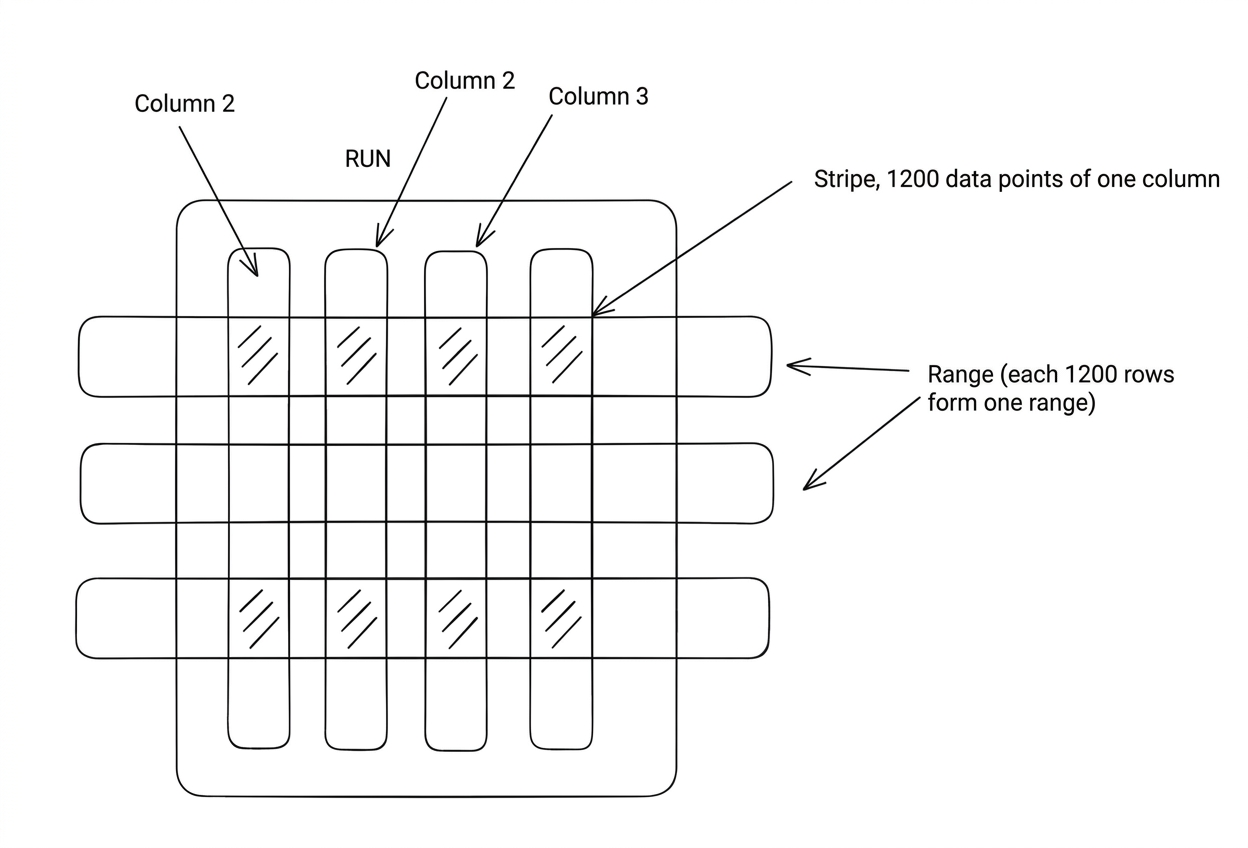
Every compress_threshold (default 1200) rows of data is called a Range. The data for a specific column within a Range (containing compress_threshold rows) is called a Stripe. If the data for a column is particularly large, the Stripe is further divided into 1MB Chunks. During reads, an entire compress_threshold worth of data is not necessarily read at once.
RUN
└── range (split by rows, default 1200 rows per range)
    ├── column1 stripe (1200 datums)
    ├── column2 stripe (1200 datums)
    ├── column3 stripe (1200 datums)
    └── ...
Range: A logical row window. Every 1200 rows form a range, which is stored internally in columnar format, compressed by column.
Stripe: A physical column block. A contiguous storage block for a specific column within the 1200-row window.
Datum: The smallest unit of value. The value of a specific row and column (native unit within the PG kernel).
The reality of hybrid workloads demands that writes often occur in small batches or continuous micro-batches, while analytical queries prefer efficient columnar scans. MARS3's approach is to combine these two requirements within the same system, using RowStore and ColumnStore in combination, assigning different responsibilities at different stages:
RowStore is more geared towards writes and access to fresh data. It more readily accepts new data and is suitable for small-range reads and detailed lookups, especially for data that has just been written and not yet reorganized.
ColumnStore is more geared towards scans and aggregations. Once data is reorganized, ColumnStore significantly improves scan throughput and compression efficiency, making large-range aggregations and filtered queries more resource-efficient.
This "row-first, column-later" approach essentially allows data to first enter the system in a write-friendly form, then be gradually transformed into an analysis-friendly form in the background, enabling the normal operation of "continuous writes, continuous queries." To accommodate different scenario requirements, YMatrix supports three write modes, determined by the table-level parameters prefer_load_mode and rowstore_size:
Normal: Default mode. Newly written data is first written to RowStore Runs in L0. After accumulating to rowstore_size, it is written to ColumnStore Runs in L1. Compared to bulk mode, this incurs one extra I/O operation, making columnar conversion asynchronous rather than synchronous. Suitable for scenarios with high-frequency, small-batch writes where I/O capacity is sufficient and low latency is important.
Bulk: Batch loading mode. Suitable for low-frequency, large-batch writes. Data is written directly to ColumnStore Runs in L1. Compared to normal mode, it saves one I/O operation, making columnar conversion synchronous. Suitable for scenarios with limited I/O capacity and low latency requirements for infrequent, large data loads.
Single: Data is inserted directly into RowStore, and tuples are placed directly in Shared Buffers.
Refer to Chapter 5 [Write Path Overview] for more details.
MARS3 currently supports BRIN and BTREE indexes. BTREE is suitable for transaction-oriented systems focused on "exact lookups," enabling fast positioning via row-level pointers. BRIN is suitable for large-scale analytical systems focused on "range scans," using block-level summaries to significantly reduce invalid I/O. Note: For MARS3 tables, a maximum of 16 indexes are currently allowed per table (regardless of whether they are on the same column or are BRIN/BTREE). Exceeding this limit results in an error: ERROR: IndexBuild error: too many indexes (index_am.h:162).
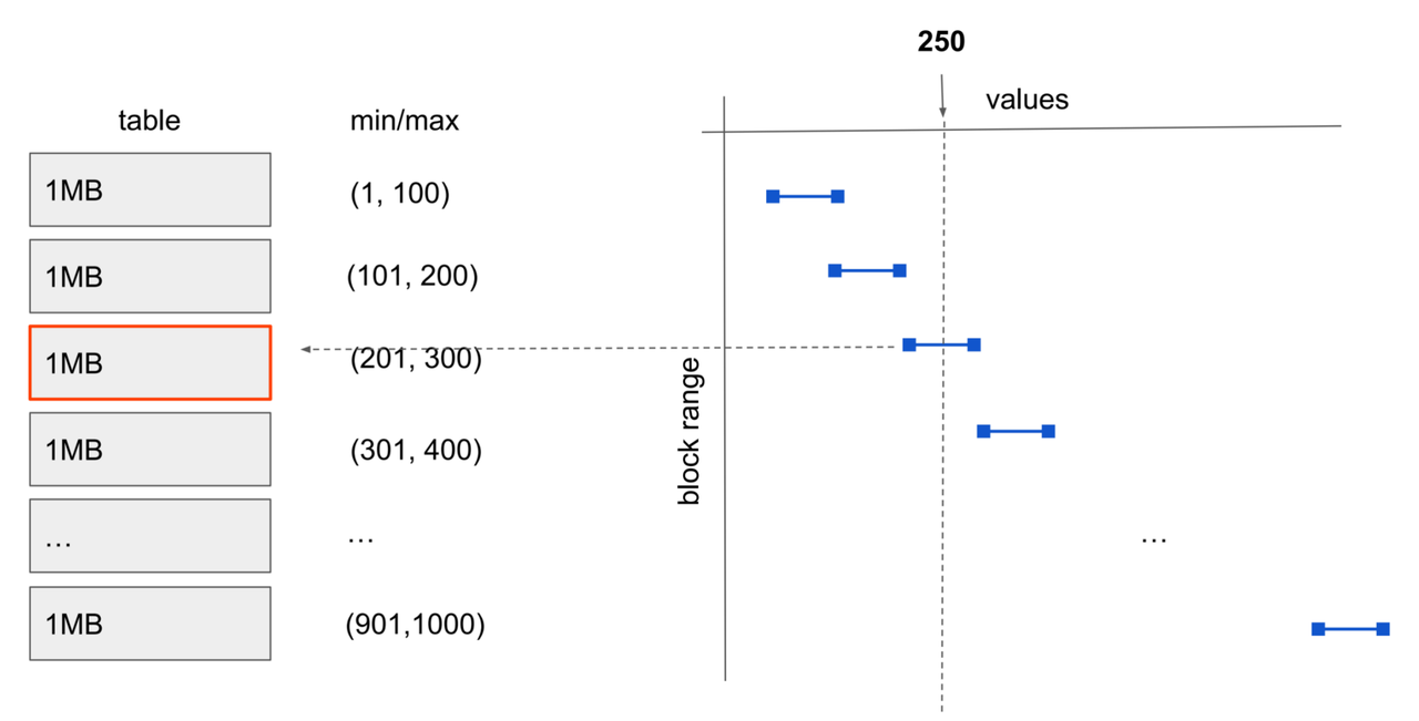
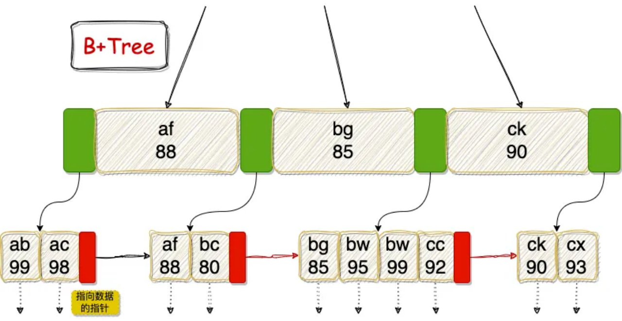
BRIN is a lightweight range-summary index designed for very large tables. Instead of pointing to specific rows, it maintains summary statistics (like minimum and maximum values) for contiguous ranges of data blocks. During query execution, it can quickly prune blocks that cannot contain matching data, significantly reducing scan I/O.
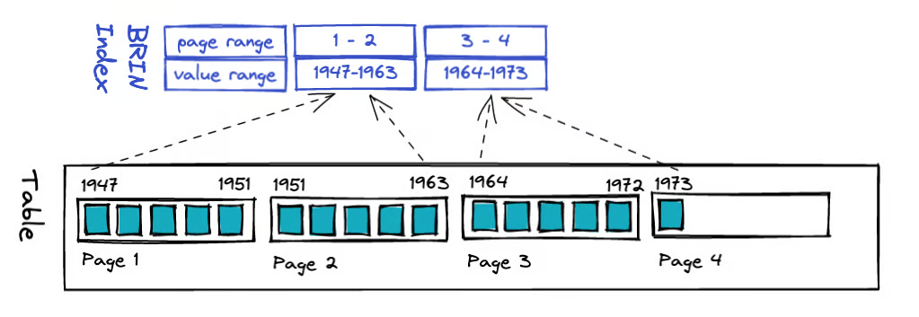
BRIN has minimal space overhead and very low build and maintenance costs. However, its effectiveness heavily depends on the physical ordering of data. When data is written in order based on a timestamp or incrementing key, BRIN can achieve scan efficiency close to partition pruning in time-series analysis and log-like scenarios. It is a valuable complementary index for large analytical tables. For example, searching for value 250 can quickly locate the third data block:
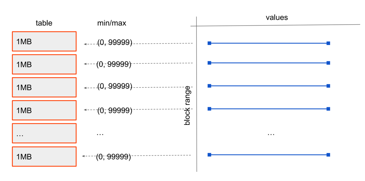
Due to the specific nature of BRIN's data structure (its core idea is maintaining summary information for contiguous data blocks, not indexing individual rows), it is not suitable for randomly distributed data or scenarios with high update frequency or frequent out-of-order updates. In such cases, BRIN degrades to a sequential scan, requiring each data block to be scanned.
YMatrix also supports [Default BRIN].
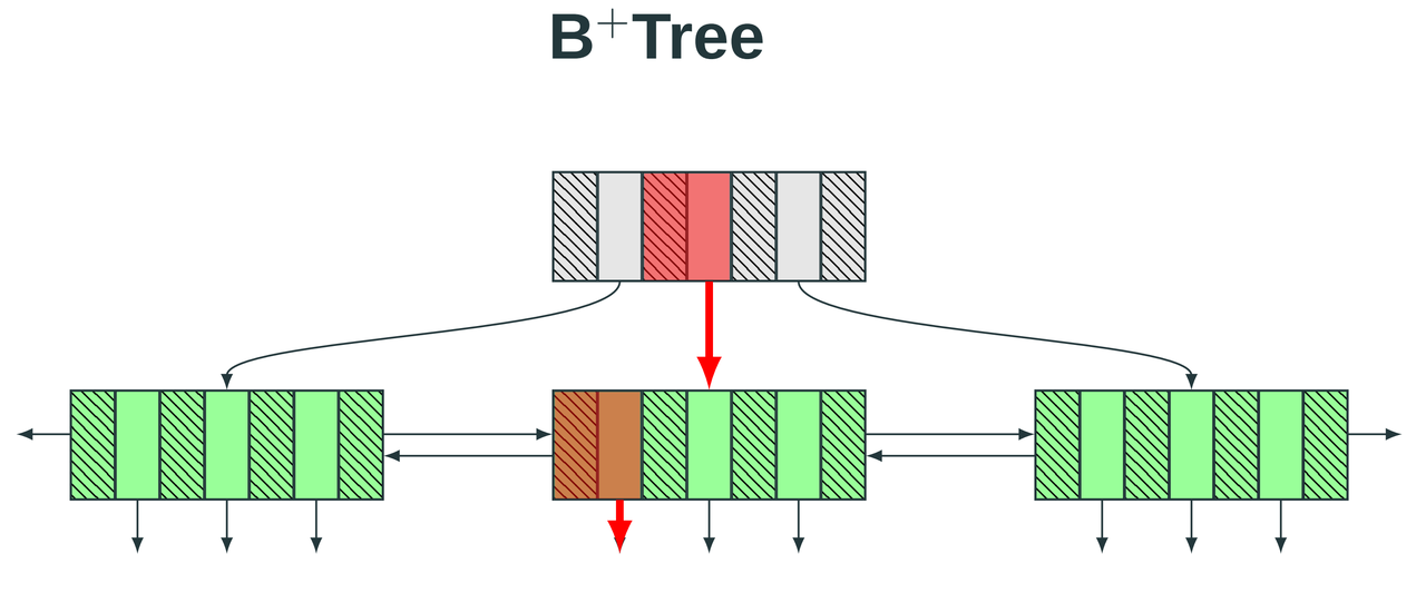
BTREE is a general-purpose index based on a balanced multi-way tree structure. It organizes index nodes by key value, enabling fast and precise location of single rows or small ranges of data. Query complexity is stable at O(logN). It supports both equality queries and efficient range scans and sorting operations. Because it does not depend on the physical distribution of data, BTREE is highly stable in high-concurrency transaction processing scenarios. It is the default index type for primary keys, unique constraints, and highly selective queries. However, it is not suitable for columns with low selectivity or wide-range scans on large tables.
mars3btree is the specialized B-tree implementation within the MARS3 storage engine. Its internal pages are standard B-tree pages. mars3btree supports two types:
NORMAL: Standard row-oriented B-tree (used for RowStore), uncompressed.
COMPRESSED: Columnar compressed B-tree (used for ColumnStore), compressed.
For columnar compressed BTREE, the overall architecture is as follows:
Min/Max Metadata: Min/max values are maintained during build and written to the metapage. The purpose is to enable global pruning before descending the btree. If the query condition falls outside the min/max range, the index can be determined as impossible to hit, acting as an ultra-lightweight directory on top of the index.
Bloom Filter: Built only for unique/primary key indexes and limited to less than 10 million entries. For point queries or existence checks on unique/primary key indexes, Bloom filters can quickly determine impossibility, reducing unnecessary leaf reads and decompression.
Fast Path Check: Enabled only for ColumnStore. A failure immediately returns nullptr, making the decision to decompress leaves a very lightweight check (min/max + bloom). If not hit, zero decompression and zero leaf reads occur.
Refer to the [Index Compression] section for syntax related to mars3btree index compression.
Similar to PostgreSQL, update and delete operations in YMatrix do not operate on the original data space in-place. Instead, they are implemented using a multi-version approach for tuples:
MARS3's update and delete operations do not modify data in place. Instead, they rely on DELTA files and version information to mask old data, controlling data visibility.
DELETE operations are recorded in the DELTA file of the corresponding Run. The data is physically removed only when the Run is merged.
UPDATE operations are implemented as a delete of the original data followed by an insert of a new row.
In MARS3, the sort key is a core design element that determines the engine's scan efficiency and long-term operational stability. Ordered data combined with reliable block-level metadata significantly enhances scan performance. A well-chosen sort key results in stronger data locality within Runs and higher levels, making query filter conditions more likely to hit contiguous ranges and enabling more effective data skipping. A poorly chosen sort key leads to more scattered data distribution, where filter conditions fail to narrow the scan range, resulting in a system that behaves like a full table scan even when indexes or metadata exist.
The core benefits of sort keys can be broken down into five categories:
Improved Filter and Range Query Efficiency: When WHERE conditions align well with the sort key (e.g., time range, device ID range), data exhibits stronger clustering at the storage layer. Queries can skip irrelevant data blocks earlier and more precisely, reducing I/O and CPU processing.
Enhanced Reliability and Data Skipping of Statistics: The value of block-level metadata like min/max and BRIN depends on data distribution. If a block contains a wide spread of key values or scattered distribution, the min/max coverage broadens, making data skipping more conservative (forcing more blocks to be read). A good sort key concentrates value ranges within blocks, making metadata more discriminative.
Influences Background Merge and Long-Term Costs: The sort key also affects Run shapes and merge effectiveness. More ordered and clustered data leads to more regular Runs after merging, making space usage and read paths more convergent. If the sort key causes data to be inherently dispersed, even merging may fail to achieve good locality, requiring more maintenance overhead to sustain performance in the long run.
Affects Compression: Compression (whether zstd/lz4 or encodings like RLE/dict/bitpack) relies on a core fact: the more regular the data within a block/stripe, the better the compression. When similar entity/time data clusters within the same stripe, intra-block value ranges narrow, repetitions and runs increase, dictionary size decreases, and bit width for delta/bitpacking reduces, enhancing the effectiveness of encoding and general compression. Refer to [Impact of Sort Keys on Compression] for validation.
Affects Write Performance: Refer to [Impact of Sort Keys on Write Performance].
Organize data based on the most common and effective filtering dimensions. In practice, sort key choices often involve a combination of two dimensions:
Time Dimension: Time-series, log, and metric workloads almost always have time range filters.
Entity Dimension: Primary key or high-frequency filtering fields for single-entity lookups like device, vehicle, user, workstation, site.
Columns frequently used in WHERE conditions should be placed earlier in the sort key.
Rule 1: Use the column with the highest occurrence frequency in WHERE filter conditions as the leftmost prefix of the sort key.
Rule 2: Place columns with high cardinality and high selectivity at the front of the sort key.
Rule 3: If using BRIN indexes, the earlier a column appears in the sort key, the more important it is – because it significantly impacts the index's ability to skip irrelevant data.
In short, aim to make the most common query conditions able to narrow the scan range to contiguous, clustered intervals as much as possible.
The following is a real customer case – a time-series scenario, with sample queries:
SELECT time_bucket_gapfill ('5 min', time) AS bucket_time,
    locf (LAST (value, time)) AS last_value,
    locf (LAST (quality, time)) AS last_quality,
    locf (LAST (flags, time)) AS last_flags
FROM
    xxx
WHERE
    id = '116812373032966284'
    AND type = 'ANA'
    AND time >= '2025-11-16 00:00:00.000'
    AND time <= '2025-11-16 23:59:59.000'
GROUP BY
    bucket_time;
The results show that different sort keys significantly impact index scan performance, working similarly to composite indexes.
Comparison of Sort Keys and Scan Performance
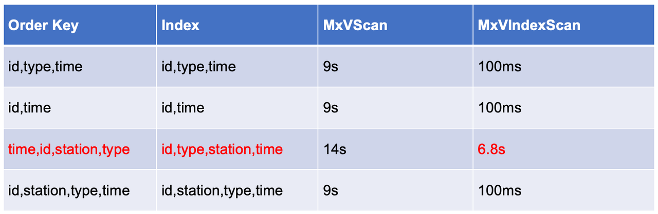
When the time field is placed first, tuples for the same ID become scattered across storage over time. Consequently, index scans need to perform many random reads to access the corresponding data blocks.
However, when ID is placed first, all tuples belonging to the same ID are stored contiguously. This drastically reduces random I/O operations because the index scan only needs to read a small number of consecutive blocks.
Data is sorted during the conversion from RowStore to ColumnStore. RowStore itself is not sorted. If a BTREE index exists on the RowStore, that BTREE index is also ordered. When a sort key is specified, the following occurs:
Keys need to be computed (retrieving column values, handling NULLs, potential type conversions/collation).
Key comparisons are needed (sorting/merging/inserting into ordered structures).
The more key columns, the more complex the types, and the more frequent the comparisons.
Not specifying a sort key typically avoids this overhead, making writes lighter. However, the sort key also affects the inherent regularity of data being written to disk:
Sorting matching the data arrival pattern → leads to more regular Runs / less subsequent rewriting → writes become more stable long-term.
Sorting mismatch → consumes more background resources (more/frequent merges) → competes for I/O and CPU → slows down foreground writes.
CREATE TABLE t_w0_nosort (
  id bigint NOT NULL,
  k1 bigint NOT NULL,   -- high cardinality
  k2 smallint NOT NULL, -- low cardinality
  k3 bigint NOT NULL,   -- monotonic column (using bigint to simulate increment)
  v1 double precision NOT NULL,
  v2 double precision NOT NULL,
  payload text NOT NULL -- to control write volume: suggest 256B/1024B
) USING mars3;

CREATE TABLE t_w1_1key (LIKE t_w0_nosort INCLUDING ALL)
USING mars3
ORDER BY (k3);

CREATE TABLE t_w3a_3key (LIKE t_w0_nosort INCLUDING ALL)
USING mars3
ORDER BY (k1, k3, k2);

CREATE TABLE t_w3b_3key (LIKE t_w0_nosort INCLUDING ALL)
USING mars3
ORDER BY (k3, k1, k2);
Building the intermediate dataset:
DROP TABLE IF EXISTS t_src_s;
CREATE TABLE t_src_s USING MARS3 AS
SELECT
  g AS id,
  (hashint8(g)::bigint) AS k1,
  (g % 64)::smallint AS k2,
  g AS k3,
  (g % 1000) * 0.01 AS v1,
  (g % 10000) * 0.001 AS v2,
  repeat('x', 256) AS payload
FROM generate_series(1, 200000000) g;

TRUNCATE t_w0_nosort;
\timing on
INSERT INTO t_w0_nosort SELECT * FROM t_src_s;
\timing off

TRUNCATE t_w1_1key;
\timing on
INSERT INTO t_w1_1key SELECT * FROM t_src_s;
\timing off

TRUNCATE t_w3a_3key;
\timing on
INSERT INTO t_w3a_3key SELECT * FROM t_src_s;
\timing off

TRUNCATE t_w3b_3key;
\timing on
INSERT INTO t_w3b_3key SELECT * FROM t_src_s;
\timing off
After completing each test, restart the database and compare the write times.
adw=# TRUNCATE t_w0_nosort;
TRUNCATE TABLE
adw=# \timing on
Timing is on.
adw=# INSERT INTO t_w0_nosort SELECT * FROM t_src_s;
INSERT 0 200000000
Time: 76859.371 ms (01:16.859)
adw=# \timing off
Timing is off.

adw=# TRUNCATE t_w1_1key;
TRUNCATE TABLE
adw=# \timing on
Timing is on.
adw=# INSERT INTO t_w1_1key SELECT * FROM t_src_s;
INSERT 0 200000000
Time: 82864.008 ms (01:22.864)
adw=# \timing off
Timing is off.

adw=# TRUNCATE t_w3a_3key;
TRUNCATE TABLE
adw=# \timing on
Timing is on.
adw=# INSERT INTO t_w3a_3key SELECT * FROM t_src_s;
INSERT 0 200000000
Time: 106929.500 ms (01:46.930)
adw=# \timing off
Timing is off.

adw=# TRUNCATE t_w3b_3key;
TRUNCATE TABLE
adw=# \timing on
Timing is on.
adw=# INSERT INTO t_w3b_3key SELECT * FROM t_src_s;
INSERT 0 200000000
Time: 83456.346 ms (01:23.456)
adw=# \timing off Throughput:
Overhead Relative to No Sort:
Placing the monotonic column k3 as the first column in the sort key reduces the write cost of multi-column sorting to nearly that of single-column sorting.
Placing the high-cardinality, random column k1 as the first column significantly increases write cost.
Why is no sort the fastest? Doing less sorting/comparison/ordering maintenance means the foreground write cost is minimized, hence it provides the baseline throughput (2.60M rows/s).
Why is ORDER BY (k3) only slightly slower? The input stream is already increasing by k3, so the sort key aligns with the input order. In most cases, writes are sequential, incurring only a small metadata maintenance overhead, hence only ~8% slower.
Why is ORDER BY (k1, k3, k2) significantly slower?
Because the sort comparison first looks at k1, which is a high-cardinality, near-random column. This scatters the entire write stream across the key space:
Makes it difficult to follow the fast path of sequential appending / local ordering.
Significantly increases the number of comparisons (multi-column comparisons + the first column almost always needs comparison to determine ordering).
More easily triggers heavier data organization tasks (buffering, merging, internal structure maintenance).
Therefore, throughput drops to 1.87M rows/s (39% slower), which is reasonable.
Because the first sort column, k3, aligns with the input stream, allowing the system to maximize the use of natural ordering:
A large number of writes are sequential in terms of k3.
k1/k2 only participate in deeper comparisons when k3 values are identical or very close, resulting in significantly less actual comparison/reshuffling pressure.
Hence, its performance is almost equivalent to ORDER BY (k3) (2.40M vs. 2.41M rows/s).
adw=# \dt+
                            List of relations
 Schema |    Name     | Type  |  Owner  | Storage |  Size   | Description
--------+-------------+-------+---------+---------+---------+-------------
 public | t_default   | table | mxadmin | mars3   | 160 kB  |
 public | t_sort_bad  | table | mxadmin | mars3   | 103 MB  |
 public | t_sort_good | table | mxadmin | mars3   | 35 MB   |
 public | t_src_s     | table | mxadmin | mars3   | 3040 MB |
 public | t_w0_nosort | table | mxadmin | mars3   | 2769 MB |
 public | t_w1_1key   | table | mxadmin | mars3   | 2764 MB |
 public | t_w3a_3key  | table | mxadmin | mars3   | 3453 MB |
 public | t_w3b_3key  | table | mxadmin | mars3   | 2764 MB |
 public | testmars3   | table | mxadmin | mars3   | 160 kB  |
(9 rows) Default BRIN is a feature of the MARS3 storage engine that provides default BRIN index support at the table level, eliminating the need for manual index creation. Unlike a regular CREATE INDEX USING BRIN (which only benefits index scans), sequential scans can also benefit from Default BRIN, significantly improving query efficiency. Note that Default BRIN does not consume index slots. Even with Default BRIN enabled, a table can still have up to 16 indexes.
| mars3_brin | mars3_default_brin | |
|---|---|---|
| Creation Method | Manual creation required | Automatically created, no manual operation needed |
| Query Support | Filters data only during IndexScan | Filters data during both IndexScan and SeqScan |
| Technical Version | brinV2 | brinV2 |
| Parameterized Query | Supports parameterized queries (param-IndexScan) | Supports parameterized queries (param-SeqScan) |
Usage syntax:
CREATE TABLE t_default(c1 bigint, c2 bigint, c3 bigint)
USING mars3 with (mars3options='default_brinkeys=30');
default_brinkeys is used to enable Default BRIN:
-1: The system automatically creates default_brin indexes for all columns that support operators <, >, =.
N: The system automatically creates default_brin indexes for the first N columns that support operators <, >, =.
postgres=# \d+ t_default
                                Table "public.t_default"
 Column |  Type  | Collation | Nullable | Default | Storage | Stats target | Description
--------+--------+-----------+----------+---------+---------+--------------+-------------
 c1     | bigint |           |          |         | plain   |              |
 c2     | bigint |           |          |         | plain   |              |
 c3     | bigint |           |          |         | plain   |              |
Distributed by: (c1)
Access method: mars3
Options: mars3options=default_brinkeys=30, compresslevel=1, compresstype=zstd
We can use a UDF to check which columns have Default BRIN:
CREATE FUNCTION matrixts_internal.mars3_brinkeys (IN r1 regclass, OUT nbrinkeys int, OUT brinkeys text)
    RETURNS SETOF RECORD
    AS '$ libdir / matrixts;', 'mars3_brinkeys'
LANGUAGE C
VOLATILE PARALLEL UNSAFE STRICT EXECUTE ON ALL SEGMENTS;

postgres=# select * from matrixts_internal.mars3_brinkeys('t_default'::regclass);
 nbrinkeys |  brinkeys
-----------+------------
         3 | (c1,c2,c3)
         3 | (c1,c2,c3)
         3 | (c1,c2,c3)
         3 | (c1,c2,c3)
(4 rows)MatrixShift for YMatrix: A Practical Guide to Migrating from Greenplum
From Greenplum to YMatrix: Migrating Core Business Data for a Leading Power-Battery Manufacturer
How a Leading ERP Vendor Entered the AI Fast Lane — A YMatrix Field Story
How MARS3 Works: Hybrid Row/Column Storage for High-Frequency Writes and Fast Analytics
Smart Manufacturing at Scale with YMatrix HTAP: Real-Time Ingestion & Unified Analytics